There is fresh movement around The Best Summer 2026 Perfumes Feature Novel Notes & Elevated Blends, and the story is worth a closer look.
We pulled together what is known so far and what it could mean for the people following it.
Summer has always been the time for fruity, fresh, and gourmand fragrances to shine — which makes perfect sense, given that it is the season of ripe berries, melty ice creams on hot days, and long walks on the beach. And while the summer 2026 perfumes continue in that tradition, with offerings heavily concentrated in those fragrance families alongside florals, they’re doing so with novel notes and unusual blends.
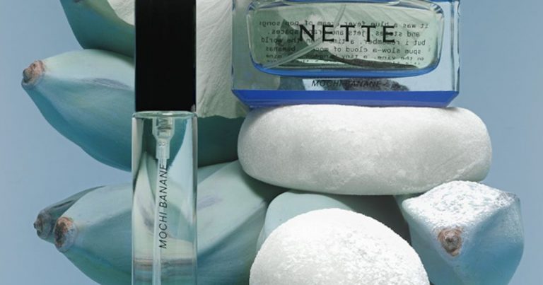
Take, for instance, Nette’s Mochi Banane, which stars a lesser-known varietal (blue) of one of fragrance’s lesser-used fruits (banana) alongside mochi and rice milk. There’s also Dior Paradise, a blend of almond and citrus notes that, as described by the brand’s perfume creation director Francis Kurkdjian, “offers a mouthwatering treat, like an irresistible almond biscuit.” Miu Miu’s Fleur de Lait combines the lactonic — specifically coconut milk — with the tropical vibes of mango, and BORNTOSTANDOUT’s Cola Addict brings everyone’s favorite non-alcoholic beverage order to your pressure points.
But that’s not to say the season is without woody, earthy, and floral offerings: There’s Coty’s Encore Une Fois L'Osmium Extrait, a warm, balsamic take on vanilla; “Gelée by Vacation,” which gives the clove and patchouli-scented sunscreen a zest of citrus; and Bvlgari’s serene black tea scent, Eau Parfumée Thé Impérial Eau de Toilette, to name a few.
Ready to dive headfirst into the best new scents of summer 2026? Keep reading to discover them.
The fragrance equivalent of cracking open an ice-cold soda on a hot day, BORNTOSTANDOUT’s Cola Addict features a sparkling blend of spicy and citrus notes, with just a hint of florals. Rum at the heart and base notes like caramel and sandalwood keep things from feeling too carbonated. | Featured notes: Cola, rum, lime, cinnamon bark
Coty’s Encore Une Fois L'Osmium Extrait de Parfum is the perfect vanilla fragrance for people who swear they don’t like vanilla fragrances. Woody and resin notes — including Peru balsam extract, labdanum, and lots of amber — create a rich and sumptuous vibe that’s anything but overly sweet. | Featured notes: Vanilla extracts, Peru balsam extract, labdanum, amber triple fusion accord, ambery woods accord
Inspired by founder Carol Han Pyle’s childhood in Hawaii, Nette’s Mochi Banane is a warm gourmand that feels like eating a not-too-sweet dessert on the beach. It opens on a creamy, slightly floral note before drying down to a cozy, earthy blend that includes sandalwood and tonka bean. | Featured notes: Blue banana, mochi accord, white Hawaiian hibiscus, rice milk, vanilla.
Inspired by Christian Dior’s Château de la Colle Noire — specifically, the designer’s “desire to see hundreds of almond trees growing there” — this woody gourmand bears the softest touch of sweetness. “The bitter almond is rarely highlighted in perfumery,” says Kurkdjian. “I paired it with a cocktail of cheerful citrus fruit top notes… which light up the entire composition.” | Featured notes: Orange, lime, mandarin, bitter almond, tonka bean
Cherry might not be everyone’s bag (pun intended), but Coach’s Cherry might be the most crowd-pleasing approach to the note yet, thanks to its blend of jasmine sambac and the woody ambrofix. The resulting fragrance is feminine, grounded, and far from syrupy. | Featured notes: Cherry, jasmine sambac, ambrofix
Lancôme’s latest fruity twist on one of its signature scents (following the sparkling raspberry La Vie est Belle and Idôle Peach ‘N Roses Eau de Parfum), La Vie est Belle Very Cherry blends the juicy stone fruit with warm and floral notes to create an elegant, ladylike fragrance. | Featured notes: Black cherry accord, violet leaf absolute, warm oud accord
Miu Miu’s latest is an easy-to-layer lactonic that smells light and summery. While it opens with mixed-drink vibes thanks to the mango and coconut, the dry-down leaves you with a fresher fragrance. | Featured notes: Mango, coconut milk, osmanthus
Viktor&Rolf’s Bonbon franchise gets in on the raspberry trend with Jelly Eau de Parfum. While the raspberry and jelly give this scent an undeniable playful sweetness, blackcurrant and peony add floral lightness that keeps things grown-up. | Featured notes: Peony, raspberry, blackcurrant
Vacation’s claim to fame is making sunscreen smell like a fine fragrance (via its original Classic Lotion). But with Gelee, it’s making fine fragrance smell like sunscreen —specifically, the beloved Orange Gelee of the 1980s. This juice updates the original earthy scent with a dash of citrusy “Zeste Méditerranéen.” | Featured notes: Bergamot, clove, saffron, patchouli, lemon, rose, sandalwood
Botanical with a healthy dash of citrus, Bvlgari’s Eau Parfumée Thé Impérial is the kind of tranquil scent that brings relaxing vacation vibes to your everyday — fitting, as the scent debuted with the brand’s hotel collection in 2017 before its release to consumers this year. | Featured notes: Sri Lankan black tea, Italian citrus (lemon, mandarin, bergamot)
America One 31 was actually the first Krigler fragrance formulated in the United States— and a favorite of Ernest Hemingway and JFK. It gets a bit of an update with Nouvelle Édition, which maintains the woody, spicy scent profile but utilizes a higher concentration of natural ingredients. | Featured notes: Bergamot, mandarin, black pepper, cedarwood, oakmoss, white musks
“Summer” may conjure up images of sweltering, sun-drenched days, but for much of the country, there are just as many rainy ones. Future Society’s Wandering Rain bottles up the precipitation itself — and not just the scent it leaves behind — with a mix of fruity, green, and floral notes. | Featured notes: Eucalyptus, citrus, pear, blue lotus, black tea, soft musks, violet