The topic Sparklines in Excel: The fastest way to visualize data without charts is currently the subject of lively discussion — readers and analysts are keeping a close eye on developments.
This is taking place in a dynamic environment: companies’ decisions and competitors’ reactions can quickly change the picture.
I relied on full Excel charts for years, but they often felt like overkill for simple tracking. Then I discovered sparklines—and suddenly I could see trends directly inside the cells. My spreadsheets became tidier, I stopped wasting time inserting and formatting complex charts, and I didn’t have to juggle floating objects.
Because sparklines squeeze a lot of information into a single cell, uneven time intervals, non-numeric entries, or cramped rows can distort your trends. That’s why it’s important to prepare your data before creating them.
It also helps to understand the basic structure you’re working with: sparklines can either summarize a single dataset as a single trend or compare multiple items across the same time period (one sparkline per row).
Once your data is ready, you can choose the right sparkline type for your use case.
Microsoft 365 includes access to Office apps like Word, Excel, and PowerPoint on up to five devices, 1 TB of OneDrive storage, and more.
Before you insert anything, decide which sparkline best fits your data. Each type visualizes a different pattern.
Line sparklines connect values with a continuous line, making them ideal for time-based patterns like monthly performance or growth trends. Use them when you need to see direction and movement rather than isolated comparisons.
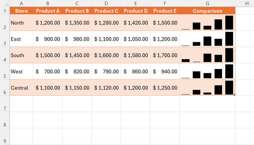
Column sparklines convert values into vertical bars, making differences in size instantly visible. They work best when comparing categories side by side.
Win/loss sparklines ignore magnitude entirely and only show whether values are positive, negative, or zero, making them ideal for streaks and binary outcomes.
Excel lets you refine sparklines in two main ways: quick visual adjustments that highlight important data points, and deeper settings that control how accurately they compare across rows.
Because sparklines are so compact, important values can easily blend into the background. After selecting the cell or cells containing your sparklines, use the Sparkline tab to surface the most meaningful parts of your data. These are some of the most useful options, but take a moment to explore the other formatting controls if you need more detailed customization:
Avoid turning on too many visual options at once. Sparklines are designed for quick scanning, and excessive formatting can make trends harder—not easier—to interpret.
The advanced options control how sparklines interpret your data rather than how they look. These settings matter most when you have missing values, are working with multiple rows of data, or are comparing trends across datasets.
Line sparklines are most sensitive to missing data and scaling because they rely on continuity, while column and win/loss sparklines are less affected visually but still follow the same dataset rules.
By default, Excel scales each sparkline independently, normalizing each row to its own range, which makes cross-row comparisons unreliable when values differ significantly. for example, a sparkline showing values between 500 and 1,000 can look nearly identical to one showing values between 5,000 and 10,000 because each row is scaled to its own range.
Selecting a cell containing a sparkline and pressing Delete doesn’t work. You have to use Excel’s dedicated removal tool to wipe the cell clean:
I still use traditional charts when I need detailed analysis, but most spreadsheets don’t need full-size visuals. Sparklines are faster and cleaner, and they keep trends directly alongside the data. That said, these mini charts are only one of many ways to visualize your data in Excel—for example, you can insert PivotTables and PivotCharts for data summarization and analysis, add slicers for interactivity, and use conditional formatting for quick highlighting.